Dynamo Fractals Part II: L-Systems and Turtle Graphics

Link to Part I: http://steellworks.blogspot.com/2013/08/dynamo-fractals.html

What's an L-System?

An L-System, short for Lindenmayer System, is a string re-writing algorithm that can be used to produce strings that can then be processed to generate geometry. In a nutshell, you take a starting string, called an axiom, and a list of rewrite rules, called productions, which you use to rewrite the axiom into a new string, which can than be rewritten again and again, ad infinitum.

An example:

Axiom: A

Productions:

A → AB

B → A

0: A
1: AB
2: ABA
3: ABAAB
4: ABAABABA
5: ABAABABAABAAB
6: ABAABABAABAABABAABABA

What's Turtle Graphics?

As mentioned above, you can take a string generated from an L-System and use it to generate geometry. The most popular method of doing this is by using a cursor whose state is manipulated by the symbols in the string produced by the L-System. For fun, we can imagine that this cursor is a turtle.

The turtle has three attributes:  a location (initialized to the origin), an orientation (initialized to the X unit vector), and a pen. It can be commanded relative to the current state of these attributes:  rather than saying "draw a line from (0, 0) to (3, 0)", instead you would say "move forward 3 units while drawing". If you wanted to make a square with end points (0, 0), (3, 0), (3, 3), and (0, 3), you would say "move forward 3 units while drawing, turn 90 degrees, move forward 3 units while drawing, turn 90 degrees, move forward 3 units while drawing, turn 90 degrees, move forward 3 units while drawing".

Obviously that's a lot of text, so each command is represented by a single character:

• + = Turn left
• - = Turn right
• ^ = Pitch up
• & = Pitch down
• \ = Roll counter-clockwise
• / = Roll clockwise
• | = Turn around
• F = Move forward while drawing
• f = Move forward without drawing
• [ = Save current position and orientation
• ] = Restore saved position and orientation

The rotation commands all rotate the same amount, which is determined when the turtle is initialized. The same goes for the distance the movement commands travel.

If we were to create the same square as before using actual Turtle Graphics commands:

Rotation: 90 degrees
Movement: 3 units
Commands: F+F+F+F

How does this relate to L-Systems?

The turtle receives its commands in the form of a string of characters. Any characters which are not one of the commands are simply ignored. This means that we can use L-Systems to generate strings containing Turtle Graphics commands!

Sounds cool, I want to use these in Dynamo!

Great, because I created a Turtle Graphics package that's available for download via the Dynamo Package Manager!

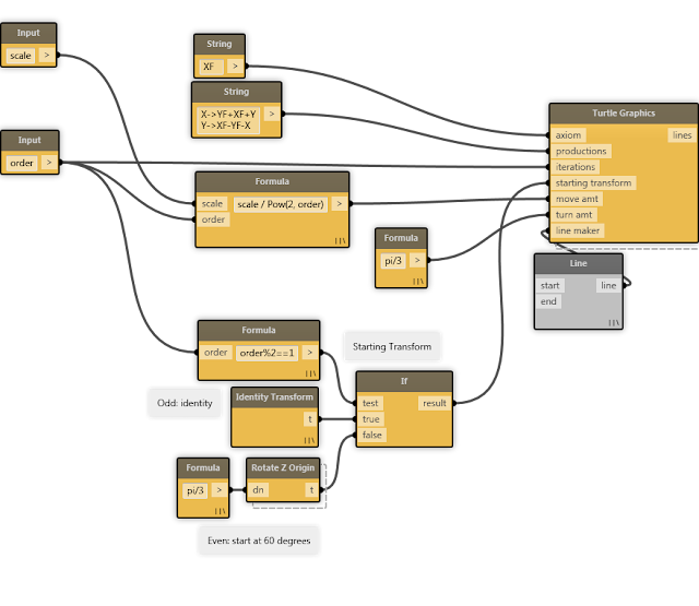
The main interface that the package provides is the Turtle Graphics node:

• start: The axiom of the L-System
• rules: Productions for the L-System
• iterations: Number of times to apply the productions to the L-system product
• initial transform: Starting transformation for the turtle
• move amt: Amount the turtle will move during the F and f commands.
• turn amt: Amount the turtle will turn during the +, -, &, ^, \, and / commands.
• line maker: Function that consumes the two end points of a line drawn with the F command. This is used to generate the output of the Turtle Graphics node.

The Turtle Graphics node returns a list of all the lines it has drawn. In order to give the user some control over how lines are represented, I've provided the line maker input, which takes a function that will receive the two end points of a line, and what it produces will be stored in the final lines list that the node will output.

For simplicity, the rules port takes the productions as a string, consisting of a list of rules separated by newlines, each composed in the following format:

[x]->[rewrite string]

(Where x is a character, and rewrite string is the string of characters to replace x with.)

Example: Sierpiński Arrowhead

Axiom: XF
Productions:
X → YF+XF+Y
Y → XF−YF−X

If you read the previous blog post, you may already understand how this is set up. We plug the axiom and productions (note the format) in as defined, iterations is plugged in from the node's order input, the starting transform is the identity transform if order is odd, and if it's true then start rotated the move amount is calculated so that the triangle's size is proportional only to the scale input (it won't scale with order.) The turn amount is set to 60 degrees.

We use the Line node as the line maker; for each line the turtle draws, Line will receive two end points (in the form of XYZs) and make a line object, which will be returned in the output list of the Turtle Graphics node.

(Note that you could use any node that can receive two XYZs in the place of the Line node, and it will change the data being output. You could, for example, plug in a List node with two input ports, and then the lines output of the Turtle Graphics node will return a list of lists that each contain two XYZs.)

"Sierpiński" example, order 8

Other Examples

Included in the Turtle Graphics package are examples of various L-Systems that you can use for reference.

"Plant" example, order 5

"Hilbert 3D" example, order 3

Dynamo Fractals

We've had a very productive and busy few days over here in the factory, but that hasn't stopped me from implementing something very dear to my heart; something I've been toying around with doing for a while now.

What's a Fractal?

Fractals are geometric constructs consisting of self-similar patterns. Most, if not all fractals are generated using simple recursive rules. It is the recursive property of a fractal's definition that gives it it's unique self-similar structure. Wikipedia has a great article, as usual.

For my Dynamo exercise, I looked for fractals which lend themselves to a simpler geometric definition rather than a pixel-by-pixel definition (such as the Mandelbrot or Julia sets). The two I decided to implement are the Sierpiński Arrowhead and the Dragon Curve. Both of these fractals start as a simple geometric figure (a line) and then on each iteration of its recursive creation, all occurrences of the original geometric figure are replaced with a new figure that contains multiple occurrences of the original figure (which can then all be replaced in the next iteration).

These fractals can both be drawn by emulating a pen: we keep track of the direction the pen is facing, and we can make the pen draw lines of a certain length in its current direction. We can turn the pen, and we can draw with the pen. These can be emulated with Transformations: turning applies a rotation to the pen's transformation, and drawing adds a translation (and the end point of the draw operation can be stored as an XYZ for creating line geometry later).

Sierpiński Arrowhead

One of the most famous fractals is the Sierpiński Triangle (also known as the Sierpiński Gasket). It's starting geometry is a solid equilateral triangle, and on each iteration an inverted equilateral triangle is removed from the center of the solid triangle, creating three solid equilateral triangles around the new hole.

The Sierpiński Arrowhead is used to approximate the whole triangle, and is useful for this exercise because it forms one complete curve (one can draw the entire Arrowhead without lifting up a pen). It's starting geometry is a line segment, that is replaced on each iteration with three line segments half the length of the original with 60 degrees between them. This replacement is inverted on every other application: the "bump" will alternate between being right-side-up and upside-down.

Based on this information, the algorithm looks like this:

Let:

• direction = direction of replacement
• length = length of each segment
• order = number of iterations to draw. Input by the user.
• scale = size of the total image. Input by the user.

In:

1. direction is initialized to upside-down. length is initialized to scale/(2^order). If order is odd, then turn 60 degrees (this will keep the triangle upright).
2. If order = 0: draw a line of length length.
3. Recur with order - 1 and direction flipped.
4. Turn 60 degrees in the current direction.
5. Recur with order - 1 and current direction.
6. Turn 60 degrees in the current direction.
7. Recur with order - 1 and direction flipped.

Step 1 is the initialization of a recursive loop, so in Dynamo all of this will be done in a node that wraps a recursive node.

The length initialization is calculated by dividing the starting scale by 2 for each iteration that will occur.

Step 2 is the start of a recursive function. All recursive calls will start there. Step 2 also represents the base case: if we started this algorithm with order as 0, then we would immediately draw a line of length scale along the X axis, which is the correct result.

Steps 3, 5, and 7 draw each of the three sub-sections of a single iteration, separated by turns in the current direction. This is exactly the definition of a single iteration of the arrowhead:  three sub-sections with 60 degrees between them. If order is 1, then the recursive calls will draw lines, and the result will be the one "bump", which is the correct result.

With that in mind, let's look at the Dynamo implementation.

At the top, we calculate the length of all drawn segments and create a translation transformation out of it. Rotation is initialized to -60 degrees. The starting transformation is set to either the identity transformation if the starting order is even, or a 60 degree rotation if the order is odd. We also initialize an accumulator that will store all of the results; since we will be storing the end-points of all the translations (emulating the draw function), we need to supply the starting point, which is the origin. All of this is passed to arrowhead curve, which contains the recursive loop.

Some notes on the inputs:

• order is the current order we are drawing
• result is the accumulated XYZs representing the end points of the drawn lines
• transform is the accumulated transformation that contains all of the translations and rotations corresponding to the draws and turns used to generate the XYZs
• translate is the pre-calculated translation used to draw the segments
• rotation is the rotation amount to be applied for turns in this iteration

If the order is 0, then we perform a draw by applying the translate to the current transform, and then applying this to an XYZ at the origin to get the appropriate XYZ. The XYZ is added to the accumulator, and the updated accumulator is returned. The updated transform with the translate applied is also returned.

If the order is not 0, the we draw the three sub-sections. We draw the first sub-section with the rotation flipped (which flips the direction). We take the result transform from the first sub-section and rotate it by the current rotation, which emulates the first turn. We pass this turned transform to the second sub-section, along with the current (non-flipped) rotation, and the results of the first sub-section. We turn the result transform again before drawing the third sub-section, which again uses the flipped rotation and the results from the second (and first) sub-section. For all three sub-sections, the order is subtracted by 1, which allows the recursion to approach the base case of order = 0. The results of the third sub-section drawing are then used as the results of the recursive branch.

Sierpinski Arrowhead in Revit, order of 7.

Dragon Curve

The Dragon Curve (also known as the Jurassic Park Curve) is another popular fractal. It is created using 45 and 90 degree angles: its starting geometry is a single line segment, and on each iteration, the single line segment is replaced by two smaller line segments of equal length joined at a 90 degree angle and oriented such that the first new segment forms a 45 degree angle with the original segment. Like the Sierpiński Arrowhead, these replacements alternate between right-side-up and upside-down.

The algorithm looks like this:

Let:

• direction = direction of replacement
• length = length of each segment
• order = number of iterations to draw. Input by the user.
• scale = size of the total image. Input by the user.

In:

1. direction is initialized to right-side-up. length is initialized to scale/2^(.5*order).
2. If order = 0: draw a line of length length.
3. Turn 45 degrees in the current direction.
4. Recur with order - 1 and direction = right-side-up.
5. Turn 90 degrees in the opposite direction.
6. Recur with order - 1 and direction = upside-down.
7. Turn 45 degrees in the current direction.

Step 1 is the initialization of a recursive loop, so in Dynamo all of this will be done in a node that wraps a recursive node.

The length initialization is calculated by dividing the starting scale by the square root of 2 for each iteration that will occur. (Square root of 2 is used because a  45-45-90 right-triangle with a hypotenuse of 1 yields a side-length of root-2 in accordance with the Pythagorean theorem).

Step 2 is the start of a recursive function. All recursive calls will start there. Step 2 also represents the base case: if we started this algorithm with order as 0, then we would immediately draw a line of length scale along the X axis, which is the correct result.

Steps 4 and 6 draw both sub-sections of a single iteration, separated by a 90 degrees turn in the opposite direction. Before and after the sub-sections are drawn, there is a 45 degrees turn in the current direction. This is exactly the definition of a single iteration of the arrowhead:  two sub-sections that form a  45-45-90 right-triangle with the original segment. The first sub-section is drawn right-side up, and the second is drawn upside-down. If order is 1, then the recursive calls will draw lines, and the result will be the one "bump", which is the correct result.

Now let's look at the Dynamo implementation.

This should look familiar if you've already seen the Sierpiński Arrowhead. At the top, we generate the translation transformation to be used for emulating draw. The transformation is initialized to the identity transform, the direction starts right-side-up, and the accumulator is initialized to contain the starting point.

Again, this should be familiar. The base case is set up identically: we perform a draw the same way as before. The recursive case is different but should be straight-forward after seeing the Arrowhead version: first we turn 45 degrees in in the current direction, then we draw the first sub-section right-side up, then we turn 90 degrees in the opposite direction, then we draw the second sub-section, and finally we turn 45 degrees in the current direction. Like last time, the accumulator and the transformation are passed along to the results.

Dragon Curve in Revit, order of 12

Dynamo: Preventing Unnecessary Evaluation (Part 2)

In my last blog post, I spoke about how we could use graph analysis in Dynamo to avoid duplicating code when compiling Dynamo workflows down to the FScheme engine. I am pleased to announce that this has now been implemented and is live on GitHub!

Of course, nothing ever goes right the first time. Hours after pushing all the new code to GitHub, during a moment of quiet reflection, I discovered why the approach I originally outlined was flawed. As with most issues in programming--I find--the problem has to do with mutation.

So what's wrong?

Let's use the following workflow as an example:

If we were to optimize this using the original approach, the resulting FScheme code would look like this:

(λ (path)
  (let ([a (read-file path)])
    (list (begin (write-file path "text")
                a
                path)
          a)))

(Note that this is a definition for a new node, so it gets compiled down to a function. Hence the λ at the beginning.)

At first glance, the problem may not seem immediately obvious. The Read File node is connected to two inputs, Perform All and List. We use the lowest single ancestor algorithm to find where we can place a let binding: in this case, it's around the List node. We evaluate the Read File node, store it in a new identifier a, and then in both places that it's used, we refer to a.

...so what's wrong?

FScheme--like most Schemes--is an eager language. This means that it will evaluate all that it can as soon as it can. When traversing the above code, first FScheme will first evaluate (read-file path) and store it in a. Then it will evaluate the body of the let binding, where (write-file path "text") will be evaluated. The problem here is that Perform All (which compiles to the begin expression) must evaluate its inputs in the order they are listed, otherwise side-effects could occur in the wrong order. Since the order in which side-effects occur matters a lot, this is a big problem.

What we really want is to not evaluate (read-file path) until we normally would, after (write-file path "text"). Then, we want to store that value somewhere and reference it later when we need it. In more traditional imperative programming languages, this is familiar. Take a look at the following snippet of C#:

delegate (string path)
{
  string a;
  writeFile(path, "text");
  a = readFile(path);
  return new List<string>() { path, a };
};

Notice how we store a after we perform writeFile, and then later we just refer to a again. Well, we can do something similar in Scheme:

(λ (path)
  (let ([a (begin)])
    (list (begin (write-file path "text")
                 (begin (set! a (read-file path))
                        a)
                 path)
          a)))

This may look strange, but we're following the same pattern as in C#:  we declare a new identifier a that's uninitialized (the (begin) code returns a value that, when used, will result in an error), then where a would normally first be referenced, we evaluate (set! a (read-file path)) which stores an actual value in a. In all other places, we can just refer to a which now contains an actual value.

Putting it all together

The full algorithm is as follows:

1. For each node X that has multiple outputs connected:
1. Assign a unique string ID to be used as a storage variable
2. Look up the lowest single ancestor LSA(X)
2. Compile the dynamo graph starting from the entry point (node with no connected output).
1. When reaching LSA(X), insert a let binding, binding ID to a (begin)
2. The first time X is reached, insert a begin that first binds the compiled form of X to ID, and then returns ID.
3. All subsequent times X is reached, simply insert ID

Dynamo: Preventing Unnecessary Evaluation

Hello again! Today I'm pleased to present some progress with automatic removal of duplicate code, an issue that has plagued Dynamo workflows for a long time.

What's the problem?

Take a look at the following workflow:

Notice that several of the nodes in the workflow have their outputs connected to multiple places. Therein lies the heart of the problem: as a user, one would expect the output of a node to be passed to all inputs connected to it. Dynamo does this, but up until now, it did this by duplicating code.

You can see this in the compiled form of the above workflow:

(list (+ (square 3) 3)
      (+ (square 3) 3) 
      (* (square 3) (square 4)) 
      (+ (square 4) (square 4)))

When Dynamo evaluates this expression, it will run all of the duplicated code: (square 3)for example, will be run 3 times. This is two more times than necessary.

That doesn't seem like big deal

It's true that for basic calculations such as in this example, the code that's duplicated doesn't make a big difference. However, if the code that's duplicated takes a long time to run--or worse, performs a mutation such as adding geometry to a Revit document--then the duplication turns out to be a very big deal.

Fortunately there was a way to work around this: the only nodes where duplication never really mattered were ones that had no inputs themselves, such as numbers or variables. This is because it's just as fast to "calculate" the output of these nodes as it would be to lookup a cached result. So what you could do is create a new node and pass in the results you want to cache as inputs. The results are then cached as the node's variables, and then you can access them as many times as you like.

To remove duplication from the above workflow using this method, the compiled expression would look like this:

((lambda (a)

  ((lambda (b)

     ((lambda (c)

        ((lambda (d)

           (list c c (* b d) (+ d d)))

         (square 4))) 

      (+ b a))) 

   (square a))) 

 3)

In the actual Dynamo UI, this would require four separate user-defined nodes, and is obviously too painful to have to do. Ideally, all of this would be done under the hood for us.

There is a better way

Scheme has a built-in construct called let for dealing with caching values, without having to use intermediate helper functions. Using let* (shorthand for nested lets), the above can be rewritten as:

(let* ([a 3]

       [b (square a)]

       [c (+ b a)]

       [d (square 4)])

  (list c c (* b d) (+ d d)))

It's actually significantly easier to have Dynamo generate a let* then having to create all of the intermediate functions. When passed to the underlying FScheme engine, it will eventually all be converted to these helper functions anyway.

So how does this happen?

Lots of graph analysis. When compiling the Expression used for evaluation, Dynamo will now check for duplicated code by looking for nodes with an output being used in more than one place. It figures out dependencies among these nodes (so that they are ordered properly in the let*) and calculates the extent of where the code will be used (to determine the "entry-point" of the let*).

For any node with more than one output, in order to determine where a let* will be placed, the lowest single ancestor for the node must be calculated. In graph theory, the LSA for a node v is another node l that lies on all paths from the root of a directed acyclic graph (which is what a Dynamo workflow is) to v, and none of l's descendants also have this property (otherwise the root node would always satisfy the problem). I found a great paper by Fischer and Huson outlining how to implement an LSA lookup.

Dynamo - FScheme Refactor Progress

I've been spending the past few weeks working on various improvements to FScheme, the core scripting engine of Dynamo. Originally I was focusing on performance, but I ended up adding a bunch of things to bring the language closer to actual Scheme. The core language is getting there, but the library is still missing a lot of what's in the R5RS Scheme standard.

What's FScheme?

Way back when Ian first created Dynamo, it used an event structure to notify nodes that their inputs have been evaluated. This was slow already, and the fact that it couldn't work inside of one Revit API transaction meant that each node had it's own transaction (something that present-day Dynamo does in Debug mode) meant that updates to Dynamo could take forever to propagate to Revit.

Starting in March of 2012, I began working on modifying the Dynamo engine so that the node interface could be converted to a Scheme-like expression which could then be evaluated, thus making Dynamo itself as full-featured a programming language as Scheme (in theory). In May, I committed these changes to GitHub.

FScheme began as a prototype in Python that I made in order to demonstrate that you can imperatively create Scheme expressions and then execute them. The idea is that the imperative interface could be wrapped by a GUI. I then set out to port the prototype to .NET so that it would be compatible with the Revit API and the existing Dynamo code. Originally, I was going to write the engine in C#, but after doing some research on tail call optimization in the language, I realized this wouldn't work. After doing a little more research, I came to the conclusion that F# would be the best candidate: it has full tail call optimization (even for x86) and it compiles to CLR code, meaning that it is not interpreted. The fact that F# code is callable from C# means that I could access this engine directly from the existing Dynamo code.

The problem with writing it in F# was that I didn't know anything about the language; the closest language to F# that I had used in the past was Haskell, and I had only used it briefly.  Fortunately, I found this great tutorial about writing a Scheme interpreter in F#, and--even better--the code was open source on GitHub. After doing some basic modifications to facilitate some features that Dynamo should support (with respect to performance and dynamic updating), I had a basic Scheme language that would be hidden to the end user behind Dynamo's UI.

So What's New?

It turns out that there were a ton of problems with the FScheme language outlined by the tutorial. The first problem was that lexical scope was broken and would prevent tail calls from being optimized properly. Macros were also first-class and evaluated at runtime, which on the one hand was cool because you can then pass macros as arguments just like you can pass functions, but it made writing library functions in F# a total headache. It also greatly messed up evaluating lists, since the evaluator made no distinction between a list data-structure and a syntax-list used for function calls.

After attempting to fix some of these things, I quickly realized that it would be simpler to rewrite the language from the ground up. So that's what I did. FScheme is now much closer to normal Scheme, except it retains the features I need for interoperability with Dynamo.

Unfortunately, a lot of these changes are not user-facing. Macros are now evaluated at compile-time, and so are no longer first class. Fortunately people don't usually pass if statements as arguments to functions, so this won't be missed. I also had to remove call/cc since nobody uses it and it was bogging down performance. Finally, I added a (simple) compiler that performs a bunch of optimizations and produces quick F# code.

For a basic benchmark, I ran the following expression in both the old FScheme implementation and the new one, and compared the execution times:

(begin (define counter (lambda (x) (if (<= x 0) x (counter (- x 1))))) (counter 1000000))

Avg. Old FScheme Execution Time: 5130ms

Avg. New FScheme Execution Time: 2539ms

Admittedly, this test only really benchmarks function call speed, but since that's the most common operation in FScheme, the fact that it runs over twice as fast is a significant accomplishment.

You can see all the new changes to the FScheme language in the fscheme-improvements branch on GitHub.